
You and Your R - Doing Statistics in Python
In this post, I will tell you how to do statistics in Python. I’ve been trained in statistics mostly with R, but I do a lot of fMRI analyses in Python and do not really want to switch back and forth.
Table of Contents
- Table of Contents
- Intro
- Prepare dataset
- Correlation
- One-sample t-test
- Independent sample t-test
- OLS Regression
- ANOVA
- Generalized Linear Models
- Linear Mixed Effects
Intro
We will be using several Python’s modules such as numpy, scipy and statsmodels. Numpy and scipy are standard modules. Statsmodels are shipped with anaconda, but if you somehow do not have statsmodels, install them via pip install -U statsmodels or easy_install -U statsmodels. Good news is that statsmodels allow doing statistics with R-like formulas (most of the time)!
In R we often work with dataframes. In Python, the dataframes are handled with Pandas, which by the way works fine with missing values. In case you do not have it, install it! Hint: pip install pandas should work ;)
Here is a very nice tutorial on Pandas, which I have no intention to rewrite here. It explains how to handle data in timeseries, dataframes, subsetting data, reading and writing, and many more.
Prepare dataset
#set common stuff
%matplotlib inline

import pandas as pd
import numpy as np
import scipy as sp
import statsmodels.api as sm
import statsmodels.formula.api as smf
import matplotlib.pyplot as plt
import warnings
warnings.filterwarnings("ignore")
np.set_printoptions(threshold='nan') #to print the whole array
Here I will make up a dataset. I will use two continuous variables, as well as one variable that good for nesting and one binary variable. To make sense out of it, here are the names for these variables. One continuous variable will be liking ice cream (just because I love it!) on a scale from 0 to 100 (hate to love respectively). It may be our dependent variable. The other continuous variable: the temperature of the weather, nesting variable is for the cities where the data were collected, and the last binary variable is for having kids. Please keep in mind, I’m not going to decipher what each model told us about the variables or whether it makes sense to run them together in a model. My goal is to show that we can run a variety of models in python, and the results will be identical to an output from R.
#generate correlated data
xx = np.array([-30.0, 110.0])
yy = np.array([0., 1000.0])
means = [xx.mean(), yy.mean()]
stds = [xx.std() / 10, yy.std() / 10]
corr = 0.7 # correlation
covs = [[stds[0]**2 , stds[0]*stds[1]*corr],
[stds[0]*stds[1]*corr, stds[1]**2]]
m = np.random.multivariate_normal(means, covs, 2500).T
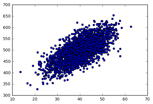
plt.scatter(m[0], m[1])
# categorical variable
cities = np.random.randint(0, 50, 2500,dtype='i')

# binary variable
kids =  np.random.randint(0, 2, 2500,dtype='i')
# Convert to Pandas. Here to make sense of all the models below, I made up some variable names.
df = pd.DataFrame({'ice_cream':m[1], 'temp': m[0], 'cities': cities, 'kids': kids})
# Assuming different cities have different preferences
for num in xrange(50):
df['ice_cream'][df['cities']==num] += df['temp']*num
# Assuming liking ice cream is increased with kids (1; no kids = 0)
df['ice_cream'][df['kids']==1] += df['temp']*1.5
# scale
df['ice_cream'] = df['ice_cream']/35
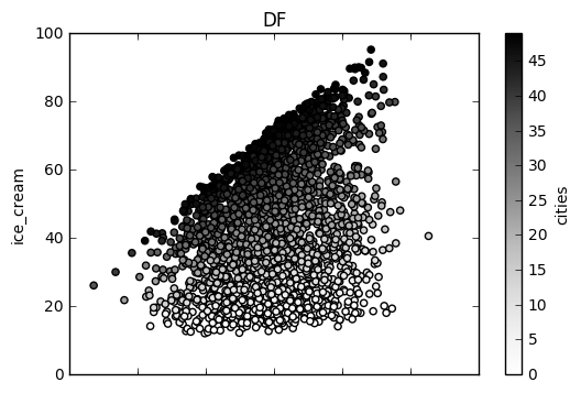
# Here is how to plot the df
df.plot(x='temp', y='ice_cream', kind='scatter', c='cities', ax=None, subplots=False, sharex=None, sharey=False,
layout=None, figsize=None, use_index=True, title='DF', grid=None, legend=True, style=None,
logx=False, logy=False, loglog=False, xticks=None, yticks=None, xlim=None, ylim=None, rot=None,
fontsize=None, colormap=None, table=False, yerr=None, xerr=None, secondary_y=False, sort_columns=False)
#Preview the top few lines
df.head()
| cities | ice_cream | kids | temp | |
|---|---|---|---|---|
| 0 | 19 | 47.529669 | 1 | 57.004601 |
| 1 | 42 | 67.420913 | 0 | 42.419001 |
| 2 | 42 | 61.912708 | 0 | 39.236830 |
| 3 | 32 | 50.251380 | 1 | 38.797294 |
| 4 | 16 | 34.368304 | 1 | 41.432471 |
# Summary
df.describe()
| cities | ice_cream | kids | temp | |
|---|---|---|---|---|
| count | 2500.000000 | 2500.000000 | 2500.00000 | 2500.000000 |
| mean | 24.492000 | 42.867872 | 0.48960 | 39.899549 |
| std | 14.563366 | 17.665057 | 0.49999 | 6.889043 |
| min | 0.000000 | 12.006117 | 0.00000 | 13.531745 |
| 25% | 12.000000 | 27.950608 | 0.00000 | 35.380744 |
| 50% | 24.000000 | 41.268259 | 0.00000 | 39.998665 |
| 75% | 38.000000 | 56.383082 | 1.00000 | 44.571119 |
| max | 49.000000 | 95.132215 | 1.00000 | 62.615418 |
# save it for replications in R
df.to_csv("~/exchange.csv")
Correlation
print "Pearson correlation with Pandas"
df.corr(method='pearson') #also available ‘kendall’ and ‘spearman’
Pearson correlation with Pandas
| cities | ice_cream | kids | temp | |
|---|---|---|---|---|
| cities | 1.000000 | 0.926675 | -0.016553 | -0.044868 |
| ice_cream | 0.926675 | 1.000000 | 0.034269 | 0.288360 |
| kids | -0.016553 | 0.034269 | 1.000000 | -0.017963 |
| temp | -0.044868 | 0.288360 | -0.017963 | 1.000000 |
print "Pearson correlation with Numpy"
print np.corrcoef(df['ice_cream'],df['temp'])
Pearson correlation with Numpy
[[ 1.          0.28836048]
 [ 0.28836048  1.        ]]
print "Pearson correlation with Scipy"
r, p = sp.stats.pearsonr(df['ice_cream'],df['temp'])
print "correlation coefficient: ", r, "; p-value: ", p
Pearson correlation with Scipy
correlation coefficient:  0.28836047698 ; p-value:  4.47496022458e-49
Looks like Scipy is the only way to test for significance
# Replicate in R
cities	   1.00000000	0.92667534	-0.01655296	-0.04486818
ice_cream	 0.92667534	1.00000000	0.03426892	0.28836048
kids	    -0.01655296	0.03426892	1.00000000	-0.01796342
temp	    -0.04486818	0.28836048	-0.01796342	1.00000000
One-sample t-test
We’ll be using the same dataframe from above.
# Using scipy
t, p = sp.stats.ttest_1samp(df['ice_cream'], popmean=0)
print "t-value: ", t, "; p-value: ", p
t-value: 121.335222203 ; p-value: 0.0
# Replicate in R

	One Sample t-test

data:  df$ice_cream
t = 121.34, df = 2499, p-value < 2.2e-16
alternative hypothesis: true mean is not equal to 0
95 percent confidence interval:
 42.17508 43.56067
sample estimates:
mean of x
 42.86787
Independent sample t-test
# With scipy
t, p = sp.stats.ttest_ind(df['ice_cream'],df['temp'])
print "t-value: ", t, "; p-value: ", p
t-value: 7.82751207811 ; p-value: 6.03132649935e-15
# With statsmodels that also give degrees of freedom
t, p, df = sm.stats.ttest_ind(df['ice_cream'],df['temp'])
print "t-value: ", t, "; p-value: ", p, "; df: ", df
t-value: 7.82751207811 ; p-value: 6.03132649935e-15 ; df: 4998.0
# Statsmodels with an unequal variance that is a default in R
# Using numpy arrays since df gives an error

t, p, df = sm.stats.ttest_ind(np.asarray(df['ice_cream']),np.asarray(df['temp']),
                              alternative='two-sided', usevar='unequal')
# alternative also accepts 'larger' and 'smaller' as one-sided indications
print "t-value: ", t, "; p-value: ", p, "; df: ", df
t-value: 7.82751207811 ; p-value: 6.68488304875e-15 ; df: 3241.93905035
# Replicate in R

	Welch Two Sample t-test

data:  df$ice_cream and df$temp
t = 7.8275, df = 3241.9, p-value = 6.685e-15
alternative hypothesis: true difference in means is not equal to 0
95 percent confidence interval:
 2.224794 3.711851
sample estimates:
mean of x mean of y
 42.86787  39.89955
OLS Regression
# Finally using an R-like formula :)
lm = smf.ols('ice_cream ~ temp',data=df).fit()
print lm.summary()
                            OLS Regression Results
==============================================================================
Dep. Variable:              ice_cream   R-squared:                       0.083
Model:                            OLS   Adj. R-squared:                  0.083
Method:                 Least Squares   F-statistic:                     226.6
Date:                Tue, 25 Oct 2016   Prob (F-statistic):           4.47e-49
Time:                        13:12:17   Log-Likelihood:                -10617.
No. Observations:                2500   AIC:                         2.124e+04
Df Residuals:                    2498   BIC:                         2.125e+04
Df Model:                           1
Covariance Type:            nonrobust
==============================================================================
                 coef    std err          t      P>|t|      [95.0% Conf. Int.]
------------------------------------------------------------------------------
Intercept     13.3653      1.989      6.719      0.000         9.465    17.266
temp           0.7394      0.049     15.052      0.000         0.643     0.836
==============================================================================
Omnibus:                      599.927   Durbin-Watson:                   2.017
Prob(Omnibus):                  0.000   Jarque-Bera (JB):              108.273
Skew:                           0.056   Prob(JB):                     3.08e-24
Kurtosis:                       1.987   Cond. No.                         238.
==============================================================================

Warnings:
[1] Standard Errors assume that the covariance matrix of the errors is correctly specified.
# Replicate in R

Call:
lm(formula = ice_cream ~ temp, data = df)

Residuals:
   Min     1Q Median     3Q    Max
-37.10 -14.21  -0.45  14.40  41.70

Coefficients:
            Estimate Std. Error t value Pr(>|t|)
(Intercept) 13.36530    1.98908   6.719 2.25e-11 ***
temp         0.73942    0.04913  15.052  < 2e-16 ***
---
Signif. codes:  0 ‘***’ 0.001 ‘**’ 0.01 ‘*’ 0.05 ‘.’ 0.1 ‘ ’ 1

Residual standard error: 16.92 on 2498 degrees of freedom
Multiple R-squared:  0.08315,	Adjusted R-squared:  0.08278
F-statistic: 226.6 on 1 and 2498 DF,  p-value: < 2.2e-16
#Now using kids as a factor in an interaction
lm2 = smf.ols('ice_cream ~ temp * C(kids)',data=df).fit()
print lm2.summary()
                            OLS Regression Results
==============================================================================
Dep. Variable:              ice_cream   R-squared:                       0.087
Model:                            OLS   Adj. R-squared:                  0.086
Method:                 Least Squares   F-statistic:                     79.05
Date:                Tue, 25 Oct 2016   Prob (F-statistic):           7.53e-49
Time:                        13:15:08   Log-Likelihood:                -10612.
No. Observations:                2500   AIC:                         2.123e+04
Df Residuals:                    2496   BIC:                         2.126e+04
Df Model:                           3
Covariance Type:            nonrobust
=====================================================================================
                        coef    std err          t      P>|t|      [95.0% Conf. Int.]
-------------------------------------------------------------------------------------
Intercept            17.2132      2.800      6.147      0.000        11.722    22.705
C(kids)[T.1]         -7.8929      3.972     -1.987      0.047       -15.683    -0.103
temp                  0.6262      0.069      9.080      0.000         0.491     0.761
temp:C(kids)[T.1]     0.2328      0.098      2.372      0.018         0.040     0.425
==============================================================================
Omnibus:                      606.961   Durbin-Watson:                   2.011
Prob(Omnibus):                  0.000   Jarque-Bera (JB):              108.752
Skew:                           0.057   Prob(JB):                     2.43e-24
Kurtosis:                       1.985   Cond. No.                         619.
==============================================================================

Warnings:
[1] Standard Errors assume that the covariance matrix of the errors is correctly specified.
# Replicate in R

Call:
lm(formula = ice_cream ~ temp * kids, data = df)

Residuals:
    Min      1Q  Median      3Q     Max
-37.481 -14.184  -0.603  14.247  40.521

Coefficients:
            Estimate Std. Error t value Pr(>|t|)
(Intercept) 17.21324    2.80043   6.147 9.19e-10 ***
temp         0.62622    0.06897   9.080  < 2e-16 ***
kids1       -7.89288    3.97245  -1.987   0.0470 *
temp:kids1   0.23279    0.09812   2.372   0.0177 *
---
Signif. codes:  0 ‘***’ 0.001 ‘**’ 0.01 ‘*’ 0.05 ‘.’ 0.1 ‘ ’ 1

Residual standard error: 16.89 on 2496 degrees of freedom
Multiple R-squared:  0.08677,	Adjusted R-squared:  0.08567
F-statistic: 79.05 on 3 and 2496 DF,  p-value: < 2.2e-16
More info http://statsmodels.sourceforge.net/stable/examples/notebooks/generated/ols.html
ANOVA
table = sm.stats.anova_lm(lm, typ=2) # Type 2 ANOVA DataFrame
print table
                 sum_sq      df           F        PR(>F)
temp       64843.702800     1.0  226.551244  4.474960e-49
Residual  714979.828862  2498.0         NaN           NaN
# Replicate in R

              Df Sum Sq Mean Sq F value Pr(>F)
temp           1  64844   64844   226.6 <2e-16 ***
Residuals   2498 714980     286
Generalized Linear Models
mod1 = smf.glm('kids ~ ice_cream', data=df, family=sm.families.Binomial()).fit()
print mod1.summary()
                 Generalized Linear Model Regression Results
==============================================================================
Dep. Variable:                   kids   No. Observations:                 2500
Model:                            GLM   Df Residuals:                     2498
Model Family:                Binomial   Df Model:                            1
Link Function:                  logit   Scale:                             1.0
Method:                          IRLS   Log-Likelihood:                -1730.9
Date:                Tue, 25 Oct 2016   Deviance:                       3461.7
Time:                        13:36:46   Pearson chi2:                 2.50e+03
No. Iterations:                     6
==============================================================================
                 coef    std err          z      P>|z|      [95.0% Conf. Int.]
------------------------------------------------------------------------------
Intercept     -0.2081      0.105     -1.979      0.048        -0.414    -0.002
ice_cream      0.0039      0.002      1.713      0.087        -0.001     0.008
==============================================================================
# Replicate in R

Call:
glm(formula = kids ~ ice_cream, family = "binomial", data = df)

Deviance Residuals:
   Min      1Q  Median      3Q     Max
-1.241  -1.157  -1.114   1.195   1.246

Coefficients:
             Estimate Std. Error z value Pr(>|z|)
(Intercept) -0.208145   0.105173  -1.979   0.0478 *
ice_cream    0.003884   0.002268   1.713   0.0868 .
---
Signif. codes:  0 ‘***’ 0.001 ‘**’ 0.01 ‘*’ 0.05 ‘.’ 0.1 ‘ ’ 1

(Dispersion parameter for binomial family taken to be 1)

    Null deviance: 3464.7  on 2499  degrees of freedom
Residual deviance: 3461.7  on 2498  degrees of freedom
AIC: 3465.7

Number of Fisher Scoring iterations: 3
More info: http://statsmodels.sourceforge.net/stable/glm.html and http://statsmodels.sourceforge.net/devel/contrasts.html
Linear Mixed Effects
# Cold ratings are nested into brands, there is only one random slople - intercept
model1 = sm.MixedLM.from_formula("ice_cream ~ temp", data=df, groups=df["cities"]).fit(reml=False)
print model1.summary()
          Mixed Linear Model Regression Results
========================================================
Model:            MixedLM Dependent Variable: ice_cream
No. Observations: 2500    Method:             ML
No. Groups:       50      Scale:              10.0311
Min. group size:  38      Likelihood:         -6609.5008
Max. group size:  70      Converged:          Yes
Mean group size:  50.0
--------------------------------------------------------
              Coef.  Std.Err.   z    P>|z| [0.025 0.975]
--------------------------------------------------------
Intercept      8.921    2.360  3.780 0.000  4.296 13.547
temp           0.851    0.009 91.185 0.000  0.833  0.869
Intercept RE 271.356   17.322
========================================================
# Replicate in R

Linear mixed model fit by maximum likelihood  ['lmerMod']
Formula: ice_cream ~ temp + (1 | cities)
   Data: df

     AIC      BIC   logLik deviance df.resid
 13227.0  13250.3  -6609.5  13219.0     2496

Scaled residuals:
    Min      1Q  Median      3Q     Max
-4.5515 -0.5695 -0.0070  0.5589  3.7772

Random effects:
 Groups   Name        Variance Std.Dev.
 cities   (Intercept) 271.35   16.473
 Residual              10.03    3.167
Number of obs: 2500, groups:  cities, 50

Fixed effects:
            Estimate Std. Error t value
(Intercept) 8.921509   2.360016    3.78
temp        0.851126   0.009334   91.19

Correlation of Fixed Effects:
     (Intr)
temp -0.158
model2 = sm.MixedLM.from_formula("ice_cream ~ temp", data=df, re_formula="temp", groups=df["cities"]).fit(reml=False)
print model2.summary()
              Mixed Linear Model Regression Results
=================================================================
Model:               MixedLM    Dependent Variable:    ice_cream
No. Observations:    2500       Method:                ML
No. Groups:          50         Scale:                 1.8684
Min. group size:     38         Likelihood:            -4551.3137
Max. group size:     70         Converged:             Yes
Mean group size:     50.0
-----------------------------------------------------------------
                       Coef.  Std.Err.   z    P>|z| [0.025 0.975]
-----------------------------------------------------------------
Intercept               8.599    0.173 49.774 0.000  8.261  8.938
temp                    0.862    0.060 14.433 0.000  0.745  0.980
Intercept RE            0.151    0.412
Intercept RE x temp RE -0.164    0.073
temp RE                 0.178    0.026
=================================================================
# Replicate in R

Linear mixed model fit by maximum likelihood  ['lmerMod']
Formula: ice_cream ~ temp + (1 + temp | cities)
   Data: df

     AIC      BIC   logLik deviance df.resid
  9114.6   9149.6  -4551.3   9102.6     2494

Scaled residuals:
     Min       1Q   Median       3Q      Max
-3.06647 -0.72209  0.01464  0.71654  2.74365

Random effects:
 Groups   Name        Variance Std.Dev. Corr
 cities   (Intercept) 0.1505   0.3879
          temp        0.1777   0.4216   -1.00
 Residual             1.8684   1.3669
Number of obs: 2500, groups:  cities, 50

Fixed effects:
            Estimate Std. Error t value
(Intercept)  8.59958    0.17196   50.01
temp         0.86235    0.05976   14.43

Correlation of Fixed Effects:
     (Intr)
temp -0.381
More info: http://statsmodels.sourceforge.net/stable/mixed_linear.html
Please email me your comments and questions!